Permutations

2026-08-17 Improve this page

For special families of permutations, see the named permutations page.

#Permutation matrices

For permutations $\pi,\sigma \in \symS_n,$ we think of multiplication as composition of functions, so that \[(\pi \circ \sigma)(k) = \pi(\sigma(k)) \text{ for $k \in [n].$}\] Given $\pi,$ we associate its permutation matrix, \[P_\pi = \left( \delta_{i, \pi(j)} \right)_{1 \leq i, j \leq n}.\] The permutation matrix of the composition $\pi \circ \sigma$ is $P_{\pi} P_{\sigma}.$ We follow the convention in [Kit11] and illustrate permutation matrices by letting row indices start at the bottom, as in the figure below. Throughout this page, this is the picture we have in mind when referring to permutation matrices.

Example (The permutation matrix for 18537462).

The permutation matrix $P_\pi$ associated with $\pi = [1, 8, 5, 3, 7, 4, 6, 2]$ using conventional row/column coordinates, and the convention we use. The rightmost figure is simply the graph of the function $i \mapsto \pi(i)$ (using Cartesian coordinates).

$P_\pi = \begin{pmatrix} 1 & 0 & 0 & 0 & 0 & 0 & 0 & 0 \\ 0 & 0 & 0 & 0 & 0 & 0 & 0 & 1 \\ 0 & 0 & 0 & 1 & 0 & 0 & 0 & 0 \\ 0 & 0 & 0 & 0 & 0 & 1 & 0 & 0 \\ 0 & 0 & 1 & 0 & 0 & 0 & 0 & 0 \\ 0 & 0 & 0 & 0 & 0 & 0 & 1 & 0 \\ 0 & 0 & 0 & 0 & 1 & 0 & 0 & 0 \\ 0 & 1 & 0 & 0 & 0 & 0 & 0 & 0 \\ \end{pmatrix}$

$ 8$ $ \, $ $ \bullet $ $ \, $ $ \, $ $ \, $ $ \, $ $ \, $ $ \,$ $ 7$ $ \, $ $ \, $ $ \, $ $ \, $ $ \bullet $ $ \, $ $ \, $ $ \,$ $ 6$ $\, $ $ \, $ $ \, $ $ \, $ $ \, $ $ \, $ $ \bullet $ $ \,$ $ 5$ $ \, $ $ \, $ $ \bullet $ $ \, $ $ \, $ $ \, $ $ \, $ $ \,$ $ 4 $ $ \, $ $ \, $ $ \, $ $ \, $ $ \, $ $ \bullet $ $ \, $ $ \,$ $ 3 $ $ \, $ $ \, $ $ \, $ $ \bullet $ $ \, $ $ \, $ $ \, $ $ \,$ $ 2 $ $ \, $ $ \, $ $ \, $ $ \, $ $ \, $ $ \, $ $ \, $ $ \bullet$ $ 1 $ $ \bullet $ $ \, $ $ \, $ $ \, $ $ \, $ $ \, $ $ \, $ $ \,$ $ 1 $ $ 2 $ $ 3 $ $ 4 $ $ 5 $ $ 6 $ $ 7 $ $ 8$

The Rothe diagram (named after H. A. Rothe) of a permutation $\pi \in \symS_n,$ denoted $D(\pi),$ is defined as the set \[D(\pi) \coloneqq \{(\pi_j,i) : i \lt{} j \text{ and } \pi_i \gt{} \pi_j \}.\] That is, we draw the permutation matrix for $\pi$ and strike out the boxes appearing somewhere to the right or above a dot, using our convention. This is illustrated in the figure below.

$The Rothe diagram for the permutation $\pi = [1, 8, 5, 3, 7, 4, 6, 2].$$

#Rothe diagram properties

The number of boxes in column $i$ of $D(\pi)$ equals the number of inversions involving position $i,$ i.e., $|\{j \gt{} i : \pi_j \lt{} \pi_i\}|.$ The total number of boxes is $|D(\pi)| = \inv(\pi).$

B. Gillen and J. Michala give intrinsic criteria for when a bubble diagram is a Rothe diagram [GM23]. Their characterizations use combinations of southwest, dot, popping, numbering, step-out avoiding, and empty-cell gap rules.

#Lehmer code

The Lehmer code (or inversion table) of a permutation $\pi \in \symS_n$ is the sequence $c(\pi) = (c_1, c_2, \dotsc, c_n)$ where \[c_i \coloneqq |\{j \gt{} i : \pi_j \lt{} \pi_i\}|.\] Note that $0 \leq c_i \leq n-i$ for all $i,$ and $c_i$ equals the number of boxes in column $i$ of $D(\pi).$ The map $\pi \mapsto c(\pi)$ is a bijection from $\symS_n$ to the set of sequences $(c_1, \dotsc, c_n)$ with $0 \leq c_i \leq n - i.$ In particular, $\inv(\pi) = c_1 + c_2 + \dotsb + c_n.$

Example (Lehmer code).

For $\pi = [1,8,5,3,7,4,6,2],$ we compute $c(\pi) = (0,6,3,2,3,2,1,0).$ For instance, $c_2 = 6$ since the entries after position $2$ that are less than $\pi_2 = 8$ are $5,3,7,4,6,2,$ all six of them. Similarly, $c_3 = 3$ since $3,4,2$ are less than $\pi_3 = 5$ among the entries after position $3.$ Therefore $\inv(\pi) = 0+6+3+2+3+2+1+0 = 17.$

#Reduced words

The simple transpositions $s_1, s_2, \dotsc, s_{n-1}$ are the generators of $\symS_n,$ where $s_i$ swaps positions $i$ and $i+1.$ Every permutation $\sigma \in \symS_n$ can be written as a product $\sigma = s_{i_1} s_{i_2} \dotsm s_{i_\ell}.$ The minimum such $\ell$ is the length of $\sigma,$ denoted $\ell(\sigma),$ and equals the number of inversions $|\INV(\sigma)|.$ A product $s_{i_1} s_{i_2} \dotsm s_{i_\ell}$ achieving this minimum is called a reduced word (or reduced expression) for $\sigma.$

#Examples

Every $\sigma \in \symS_n$ satisfies $\ell(\sigma) = \inv(\sigma) = |D(\sigma)|.$

Example (Reduced words).

Consider $\sigma = [3,1,4,2].$ We have $\inv(\sigma) = 3$ (the inversions are $(1,2), (1,4), (3,4)$), so $\ell(\sigma) = 3.$ One reduced word is $s_2 s_1 s_3:$ \[[1,2,3,4] \xrightarrow{s_2} [1,3,2,4] \xrightarrow{s_1} [3,1,2,4] \xrightarrow{s_3} [3,1,4,2].\] Since $s_1$ and $s_3$ commute (they act on disjoint positions), $s_2 s_3 s_1$ is also a reduced word: \[[1,2,3,4] \xrightarrow{s_2} [1,3,2,4] \xrightarrow{s_3} [1,3,4,2] \xrightarrow{s_1} [3,1,4,2].\] These are the only two reduced words for $[3,1,4,2].$ The number of reduced words for $\sigma$ is given by the coefficient of $x_1 x_2 \dotsm x_{\ell(\sigma)}$ in the Stanley symmetric function $F_\sigma(\xvec).$

#Bruhat order and weak order

The Bruhat order (or strong order) on permutations is a partial order $\leq$ on $\symS_n.$ We have $\sigma \leq \tau$ if $\tau$ can be obtained from $\sigma$ via a sequence of transpositions, which increase the number of inversions in each step. Equivalently, $\sigma \leq \tau$ if and only if there are reduced words $w_\sigma,$ $w_\tau$ for $\sigma$ and $\tau$ such that $w_\sigma$ is a subword of $w_\tau.$

The Bruhat order is a ranked poset, with rank given by the number of inversions.

The (right) weak order is a subposet of the Bruhat order, where only simple transpositions are allowed when multiplying on the right. This corresponds to swapping adjacent entries. Let us write $\leq_R$ for this relation. Equivalently, $\sigma \leq_R \tau$ if and only if there are reduced words $w_\sigma,$ $w_\tau$ for $\sigma$ and $\tau$ such that $w_\sigma$ is a prefix of $w_\tau.$

Bruhat poset for $n=4.$

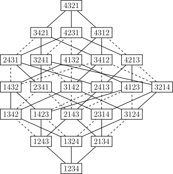
In this figure, we show the Hasse diagram of the Bruhat order for $\symS_4.$ The solid edges indicate covering relations in the (right) weak order. See [Ch. 10.5, Ful97], [Exs. 183 and 185, Sta11] and [Chs. 2–3, Bjo05] for more properties and alternative definitions.

#Braid relations

The symmetric group $\symS_n$ is generated by the simple transpositions $s_1, s_2, \dotsc, s_{n-1},$ and these generators satisfy the relations \[s_i^2 = 1,\qquad s_i s_j = s_j s_i \text{ if } |i-j| \gt{} 1,\qquad s_i s_{i+1} s_i = s_{i+1} s_i s_{i+1}.\] The last relation is called the braid relation, and together these relations give the usual Coxeter presentation of $\symS_n.$ They also explain how different reduced words for the same permutation arise: any two reduced words are connected by a sequence of commutation relations and braid relations.

For affine permutations, signed permutations, colored permutations, and Stirling permutations, see the generalizations of permutations page.

Bibliography

[Bjo05]Anders Björner. Combinatorics of Coxeter groups. Springer, 2005.

.bib

@Book{Bjorner2005,
 author = {Björner, Anders},
 title = {Combinatorics of {C}oxeter groups},
 publisher = {Springer},
 year = {2005},
 address = {New York, NY},
 isbn = {978-3-540-27596-1}
}

[Ful97]William Fulton. Young tableaux: With applications to representation theory and geometry. London mathematical society student texts (book 35). Cambridge University Press, 1997.

.bib

@book{Fulton1997,
  title = {Young Tableaux: With Applications to Representation Theory and Geometry},
  doi = {10.1017/cbo9780511626241},
  author = {William Fulton},
  isbn = {978-0511626241},
  series = {London Mathematical Society Student Texts (Book 35)},
  year = {1997},
  publisher = {Cambridge University Press}
}

[GM23]Ben Gillen and Jonathan Michala. Characterizing Rothe Diagrams. arXiv:2303.11392, 2023.

.bib

@article{GillenMichala2023x,
  author = {Ben Gillen and Jonathan Michala},
  title = {Characterizing {R}othe {D}iagrams},
  year = {2023},
  eprint = {2303.11392},
  url = {https://arxiv.org/abs/2303.11392},
  journal = {arXiv e-prints}
}

[Kit11]Sergey Kitaev. Patterns in permutations and words. Springer Berlin Heidelberg, 2011.

.bib

@book{Kitaev2011,
  doi = {10.1007/978-3-642-17333-2},
  url2 = {https://doi.org/10.1007/978-3-642-17333-2},
  year = {2011},
  publisher = {Springer Berlin Heidelberg},
  author = {Sergey Kitaev},
  title = {Patterns in Permutations and Words}
}

[Sta11]Richard P. Stanley. Enumerative Combinatorics: Volume 1. Cambridge University Press, Second, 2011.

.bib

@book{StanleyEC1,
 author = {Richard P. Stanley},
 title = {Enumerative {C}ombinatorics: {V}olume 1},
 year = {2011},
 isbn = {9781107602625},
 edition = {Second},
 doi = {10.1017/CBO9781139058520},
 publisher = {Cambridge University Press}
}